Robin O'Connell

Ray Tracing

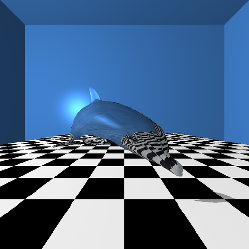
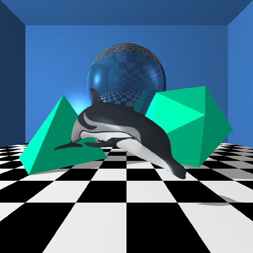
During my final semester at CSU Sacramento, I undertook an independent project for Dr. Scott Gordon concerning a 3D graphics technique called ray tracing. I extended the work of his former student—who had implemented ray tracing for geometric primitives like planes, spheres, and cubes—to accomodate arbitrary 3D models composed of tens of thousands of triangles. My work will form the basis of a new chapter in the next edition of Dr. Gordon's textbook, Computer Graphics Programming in OpenGL with Java, which has been used in 3D graphics courses at universities all around the US.

See below for more information about the techniques I studied and implemented for this project.

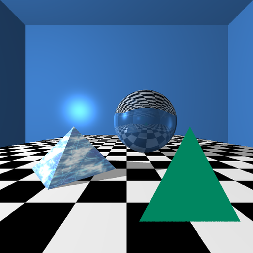
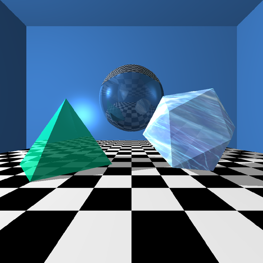
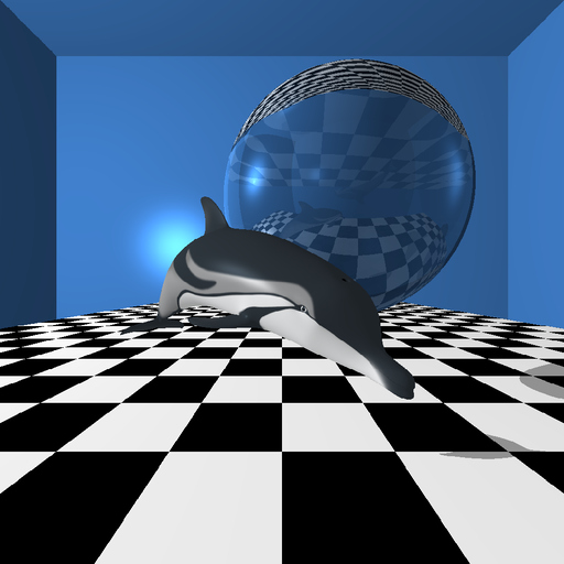
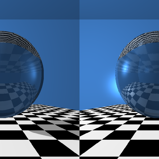
Screenshots

Tools & Technologies

Overview

Typically, 3D graphics are rendered by applying a matrix transformation that projects triangles in 3D space onto a 2D plane and then employing a rasterization algorithm that maps them to pixels on the screen. Ray tracing is an alternative approach that works by simulating the path light takes through a scene—but in reverse, starting at the "camera." Generally speaking, the matrix projection method is faster and thus better suited to realtime applications, while ray tracing is capable of heightened realism, particularly when depicting reflective and/or transparent materials such as glass.

My work can be divided into three phases: (1) rendering of individual triangles, (2) rendering of simple meshes, and (3) rendering of complex meshes.

Ray-Triangle Intersection and Vertex Attribute Interpolation

The essential strategy in ray tracing is determining where rays of light and objects in the scene intersect. Thus, my work began with implementing ray-triangle intersection. There are many approaches to this problem; I selected the well-known Möller–Trumbore algorithm for its performance and relative simplicity.

Knowing the point of intersection is only half the battle. For texturing, lighting, reflections, and refractive materials, I also needed the normal vector and texture coordinates at that point. Conveniently, the Möller–Trumbore algorithm outputs barycentric coordinates, which are expressed as a weighted average of the triangle's vertices. Hence, I could calculate the desired properties by multiplying these weights by the normals and texture coords specified for each vertex.

Mesh Serialization and Ray-Mesh Intersection

Once I could render triangles, I turned my attention to meshes. A mesh is a set of triangles (or quads) that define the surface of a 3D object. To start, I needed a way of copying the mesh data into VRAM. I packed the data for all the meshes in the scene into three long float arrays—one for vertex positions, one for normals, one for texture coords—and recorded the starting index and length of each model's data. Then, I placed the arrays into SSBOs (shader storage buffer objects), which are designed for transferring large amounts of data to the GPU. On the shader side, I could reference the starting index/length to create an instance of the model in the scene.

To test if a ray and mesh intersected, I would iterate over every triangle in the mesh and apply the algorithm from the previous section. In this manner, I was able to render simple models of up to a few hundred triangles. However, note that the cost of each ray-mesh intersection grows linearly. Furthermore, the time taken to render scenes with transparent or reflective objects grows tremendously fast—roughly O(n^k) for n triangles and recursive depth k. I needed a better method to render complex objects within a reasonable timeframe.

Bounding Volume Hierarchies

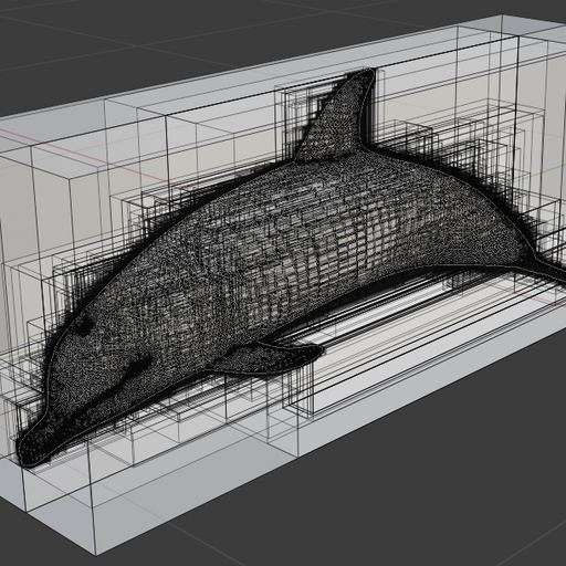
I optimized ray-mesh intersection by employing a data structure known as a bounding volume hierarchy (BVH). A BVH is a tree in which each leaf node corresponds to 1 or more triangles (or other primitives) in a mesh (or scene). Each internal node is associated with a volume (such as a cube) that contains every primitive in that subtree—hence bounding volume. The root node's bounding volume encompasses the entire object.

For example, a very simple BVH for a humanoid mesh might have 6 leaves: head, torso, left arm, right arm, left leg, right leg. The next layer up in the tree could have two nodes: upper body (head/torso/arms) and lower body (legs). Finally, the root node would encompass the whole body.

To test if a ray and mesh intersect using a BVH, start at the root node and work your way down. For each node, you only need to check its children if the ray intersects the bounding volume. If they don't intersect, you've ruled out the entire subtree with potentially vast numbers of triangles. Thus, with a well-constructed BVH, ray-mesh intersection can be reduced from linear to logarithmic time—a massive improvement when working with poly counts in the tens or hundreds of thousands.